11.3 置信区间与置信带
在这一节,根据KM估计来构建置信区间和置信带。
11.3.1 置信区间
11.3.1.1 Linear CI
记
\[ \sigma^2_S(t)=\frac{\hat V[\hat S(t)]}{\hat S^2(t)} \tag{11.30} \]
则
\[ \hat V[\hat S(t)]=\hat S(t)^2\sigma^2_S(t) \tag{11.31} \]
则可得KM估计的渐近正态分布为
\[ \frac{\hat S(t)-S(t)}{\sqrt{\hat V[\hat S(t)]}} \sim N(0,1) \tag{11.32} \]
易得\(S(t)\)在\(t_0\)时刻的\(1-\alpha\)置信区间为
\[ \hat S(t_0) \mp Z_{1-\alpha/2}\sigma_S(t_0)\hat S(t_0) \tag{11.33} \]
该区间是对称区间
11.3.1.2 Log-Transformed CI
考虑累积风险函数的对数形式\(\ln [-\ln \hat S(t_0)]\),根据\(\delta\)方法,可得其渐近分布为
\[ \ln [-\ln \hat S(t)]-\ln [-\ln S(t)] \sim N(0,\frac{\sigma_S^2(t)}{\ln^2 \hat S(t)}) \tag{11.34} \]
故\(t_0\)时刻的置信区间为
\[ \ln [-\ln\hat S(t_0)] \mp Z_{1-\alpha/2}(-\sigma_S(t_0)/\ln \hat S(t_0)) \tag{11.35} \]
\(\ln \hat S(t_0) \lt 0\)
由于我们关注\(S(t_0)\)的置信区间,则需要对该置信区间进行转化,转化后的置信区间为
\[ \begin{array}{c} \ln [-\ln \hat S(t_0)]-Z(-\frac{\sigma_S(t_0)}{\ln \hat S(t_0)}) \leq \ln [-\ln S(t_0)] \leq \ln [-\ln \hat S(t_0)]+Z(-\frac{\sigma_S(t_0)}{\ln \hat S(t_0)}) \\ -\ln \hat S(t_0) \cdot \exp\{\frac{Z\sigma_S(t_0)}{\ln \hat S(t_0)}\} \leq -\ln S(t_0) \leq -\ln \hat S(t_0) \cdot \exp\{-\frac{Z\sigma_S(t_0)}{\ln \hat S(t_0)}\} \\ -\ln \hat S(t_0) \cdot \theta \leq -\ln S(t_0) \leq -\ln \hat S(t_0) \cdot \theta^{-1} \\ \ln \hat S(t_0)^\theta \geq \ln S(t_0) \geq \ln \hat S(t_0)^{\theta^{-1}} \\ \hat S(t_0)^{\theta^{-1}} \leq S(t_0) \leq \hat S(t_0)^\theta \end{array} \tag{11.36} \]
其中\(\theta=\exp\{\frac{Z\sigma_S(t_0)}{\ln \hat S(t_0)}\}\)。
11.3.1.3 Arcsine-Square Root Transformed CI
考虑\(\arcsin\{\hat S^{\frac{1}{2}}(x)\}\),则其渐近分布为
\[ \arcsin\{\hat S^{\frac{1}{2}}(t)\}-\arcsin\{S^{\frac{1}{2}}(t)\} \sim N(0,\frac{\sigma^2_S(t)\hat S(t)}{4(1-\hat S(t))}) \tag{11.37} \]
同样也可将置信区间进行转化
\[ \begin{array}{c} L \leq \arcsin\{S^{\frac{1}{2}}(t_0)\} \leq R \\ \sin \{\max [0,L]\} \leq S^{\frac{1}{2}}(t_0) \leq \sin \{\min [\frac{\pi}{2},R]\} \\ \sin^2 \{\max [0,L]\} \leq S(t_0) \leq \sin^2 \{\min [\frac{\pi}{2},R]\} \end{array} \tag{11.38} \]
注意\(\arcsin x\)的定义域与值域
其中
\[ \begin{array}{c} L=\arcsin\{\hat S^{\frac{1}{2}}(t_0)\}-\frac{Z\sigma_S(t_0)}{2}\sqrt \frac{\hat S(t_0)}{1-\hat S(t_0)} \\ R=\arcsin\{\hat S^{\frac{1}{2}}(t_0)\}+\frac{Z\sigma_S(t_0)}{2}\sqrt \frac{\hat S(t_0)}{1-\hat S(t_0)} \end{array} \tag{11.39} \]
11.3.2 置信带
置信区间给出了\(t\)在某点处的一个\(1-\alpha\)区间。而置信带则给出了\(t\)在某个区间内的一个\(1-\alpha\)区间,即\(1-\alpha=P(L(t)\leq S(t) \leq U(t)), \; \forall t \in (t_L, t_U)\),则称区间\([L(t),U(t)]\)为置信带。
由于置信带需要查表才能得到,故不多做介绍,仅了解即可。
11.3.3 平均生存时间的置信区间
平均生存时间定义为
\[ \mu = E(x)=\int_0^\infty tf(t)dt=\int_0^\infty S(t)dt \tag{11.40} \]
利用分部积分即可转化为\(S(t)\)
故区间\([0, \tau]\)上的平均生存时间估计为
\[ \hat \mu_\tau=\int_0^\tau \hat S(t)dt \tag{11.41} \]
其中\(\tau\)是\(t_{max}\)或最大的删失值。
而\(\hat \mu_\tau\)的方差为
\[ \hat V(\hat \mu_\tau)=\sum_{i=1}^D \{[\int_{t_i}^\tau \hat S(t)dt]^2\frac{d_i}{Y_i(Y_i-d_i)}\} \tag{11.42} \]
相应的置信区间为
\[ [\hat \mu_\tau-Z_{1-\alpha/2}\sqrt{\hat V(\hat \mu_\tau)},\hat \mu_\tau+Z_{1-\alpha/2}\sqrt{\hat V(\hat \mu_\tau)}] \tag{11.43} \]
11.3.4 分位数的置信区间
生存函数的分位数定义为\(x_p = \inf\{t:S(t) \leq 1-p \}\),则\(x_p\)的km估计为\(\hat x_p=\inf\{t:\hat S(t) \leq 1-p \}\)。
进一步的,Brookmeyer和Crowley给出了分位数置信区间的三种形式。
\[ \begin{array}{c} -Z_{1-\alpha/2} \leq \frac{\hat S(t)-(1-p)}{\hat V^{1/2}[\hat S(t)]} \leq Z_{1-\alpha/2} \\ -Z_{1-\alpha/2} \leq \frac{\{\ln [-\ln (\hat S(t))]-\ln [-\ln(1-p)]\}\hat S(t)\ln (\hat S(t))}{\hat V^{1/2}[\hat S(t)]} \leq Z_{1-\alpha/2} \\ -Z_{1-\alpha/2} \leq \frac{2[arcsin(\hat S^{\frac{1}{2}}(t))-arcsin(1-p)^{\frac{1}{2}}][\hat S(t)(1-\hat S(t))]^{1/2}}{\hat V^{1/2}[\hat S(t)]} \leq Z_{1-\alpha/2} \end{array} \tag{11.44} \]
11.3.5 左截断数据的置信区间
不妨先举个例子
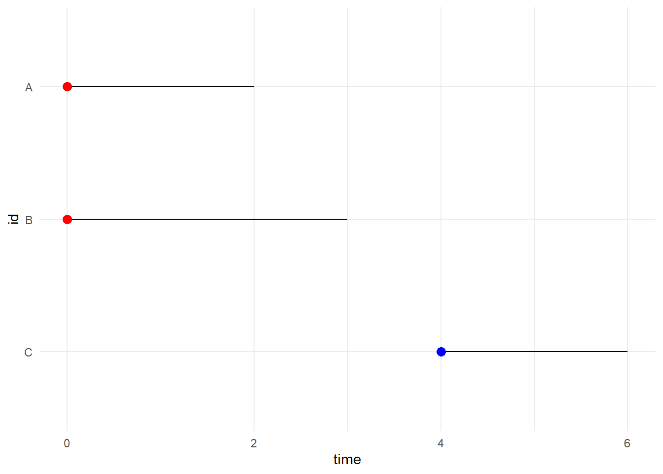
在这个例子中,A、B都是在一开始就进入到研究中的,而C是中途加进来的。也就是说,我们一开始是观测不到C的。因此在原有的计算规则下,我们有如下结果
- \(t_1=2;\; d_1=1; \; R(t_1)=\{A,B\}; \; Y_1=2; \; \hat S(t_1)=1/2\)
- \(t_2=3;\; d_2=1; \; R(t_2)=\{B\}; \; Y_2=1; \; \hat S(t_2)=0\)
- \(t_3=6;\; d_3=1; \; R(t_3)=\{C\}; \; Y_3=1; \; \hat S(t_3)=0\)
明明C能够生存到\(t_2\)之后,只是之前没有观测到,但生存函数的估计却在\(t_2\)时刻估计为0,存在一些问题。
鉴于此,我们需要拓展\(Y_i\)的定义:在\(t_i\)时刻前进入到研究中并在\(t_i\)时刻仍存活的个体,或者在\(t_i\)时刻之后进入到研究中并且其生存时长大于等于\(t_i\)的个体都会被计入。
- \(t_1=2;\; d_1=1; \; R(t_1)=\{A,B,C\}; \; Y_1=3; \; \hat S(t_1)=2/3\)
- \(t_2=3;\; d_2=1; \; R(t_2)=\{B,C\}; \; Y_2=2; \; \hat S(t_2)=1/3\)
- \(t_3=6;\; d_3=1; \; R(t_3)=\{C\}; \; Y_3=1; \; \hat S(t_3)=0\)
这样,对于生存函数的估计我们就得考虑条件概率,即\(P(X \gt t |X \geq L)=S(t)/S(L)\)。当然,当对象一开始就纳入到研究中,那么\(L=0\),按以前的操作来就行。这里只是将研究工具拓展到左截断数据。
\[ \hat S_L(t)=S(t)/S(L)=\prod_{L \leq t_i \leq t}[1-\frac{d_i}{Y_i}] \tag{11.45} \]
左截断数据需要对改变生存函数的估计,其他构造置信区间的操作同正常情况。