10.6 Seq2Seq
10.6.1 原理
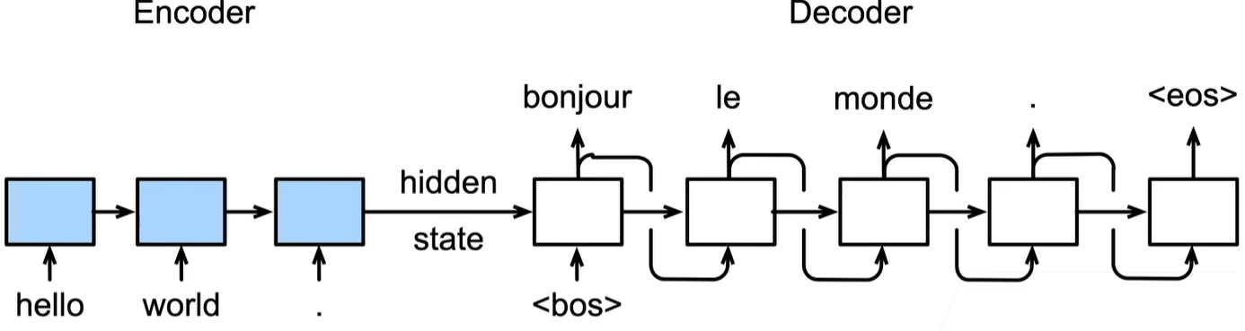
图 10.4: seq2seq
当然对于翻译任务,应当有个词嵌入环节
Seq2Seq由编码器和解码器组成,二者均是RNN(包括LSTM和GRU)结构,用于解决由原始序列输出目标序列的任务,两个序列可以不等长。
在编码器部分,由于输入序列已知,因此可以使用双向RNN结构用于提取信息,然后在最后一个时间步输出隐状态,并将此隐状态作为上下文向量context vector,记为\(c\)。
上下文向量相当于是对原始序列信息的一个浓缩
在解码器部分,若记解码器的隐状态为\(s\),则
\[ s_t = f(s_{t-1}, y_{t-1}, c) \]
即解码器t时刻的隐状态由上一步的隐状态、上一步的预测值、编码器的上下文向量共同输入得到。
在训练时,采取\(Teacher Forcing\)策略,即每次输入的\(y\)值为真实值,这有助于模型训练。但在预测时则接收上一步的预测值作为输入
但是,Seq2Seq有很明显的缺陷,即在解码器中使用的上下文向量是固定的,而由于编码器的RNN结构,导致这个上下文向量难以记住更早的重要信息。于是,提出Seq2Seq+注意力机制的方法。
下面介绍Luong的论文Effective Approaches to Attention-based Neural Machine Translation。
这篇论文可以说是对Bahdanau的NEURAL MACHINE TRANSLATION BY JOINTLY LEARNING TO ALIGN AND TRANSLATE这篇论文的改进,有细微差异,例如这篇论文用\(s_{t-1}\)来更新\(c_t\),而Luong用\(s_t\)
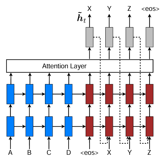
图 10.5: Seq2Seq与注意力机制(Input-Feeding)
计算流程为:
- 编码阶段
输入序列 \((x_1, x_2, \ldots, x_S)\) 经双向LSTM编码得到:
\[ h_1, h_2, \ldots, h_S = \text{EncoderRNN}(x_1, \ldots, x_S) \]
每个\(h_s\)是源序列中第\(s\)个词的隐状态输出。
- 解码器状态更新
在时间步\(t\),解码器根据上一步输出的目标词\(y_{t-1}\)与前一隐藏状态 \(s_{t-1}\),更新当前解码器状态:
\[ s_t = \text{DecoderRNN}(y_{t-1}, s_{t-1}) \]
此时 \(s_t\) 表示“当前要生成第 \(t\) 个词”的语义状态。
论文还提出了Input-Feeding机制,即在生成\(s_t\)时也用到了\(\tilde{s}_{t-1}\)的信息,\(\tilde{s}_{t-1}\)后续会介绍。
\[ s_t = \text{DecoderRNN}(y_{t-1}, \tilde{s}_{t-1}, s_{t-1}) \]
- 注意力机制
通过相似度函数计算\(s_t\)与每个\(h_s\)的匹配程度,论文中介绍了三种计算方法:
\[ \text{score}(s_t, h_s) = \begin{cases} s_t^\top h_s, & \text{(Dot)} \\ s_t^\top W_a h_s, & \text{(General)} \\ v_a^\top \tanh(W_a [s_t; h_s]), & \text{(Concat)} \end{cases} \]
Bahdanau的论文中使用\(e_{t,i}= v_a^{T} \text{tanh}(W_ss_{t-1}+W_hh_i)\)加性注意力函数来计算相似度得分
之后通过softmax归一化得到每个源词的注意力权重:
\[ a_t(s) = \frac{\exp(\text{score}(s_t, h_s))} {\sum_{s'=1}^{S} \exp(\text{score}(s_t, h_{s'}))} \]
其中\(a_t(s)\) 表示当前解码器在生成第\(t\)个词时,关注源序列\(s\)个位置的程度。
- 计算上下文向量
对编码器输出进行加权求和,得到上下文向量:
\[ c_t = \sum_{s=1}^{S} a_t(s)\, h_s \]
\(c_t\)是源端信息的加权摘要,代表模型在第\(t\)步“看到”的输入信息。
- 信息融合
Luong 定义了attentional hidden state:
\[ \tilde{s}_t = \tanh(W_c [c_t; s_t]) \]
该向量综合了当前目标语义与注意到的源端信息。
- 输出词预测
通过线性层与 softmax 计算目标词概率分布:
\[ p(y_t \mid y_{<t}, x) = \text{softmax}(W_o \tilde{s}_t) \]
取概率最大的词作为预测输出:
\[ \hat{y}_t = \arg\max_y p(y_t) \]