11.4 GRU

11.4.1 原理

GRU是LSTM的简化版本，仅有两个门控——重置门（遗忘）与更新门，同时也缺少记忆元，这使得GRU在训练时更加快捷。

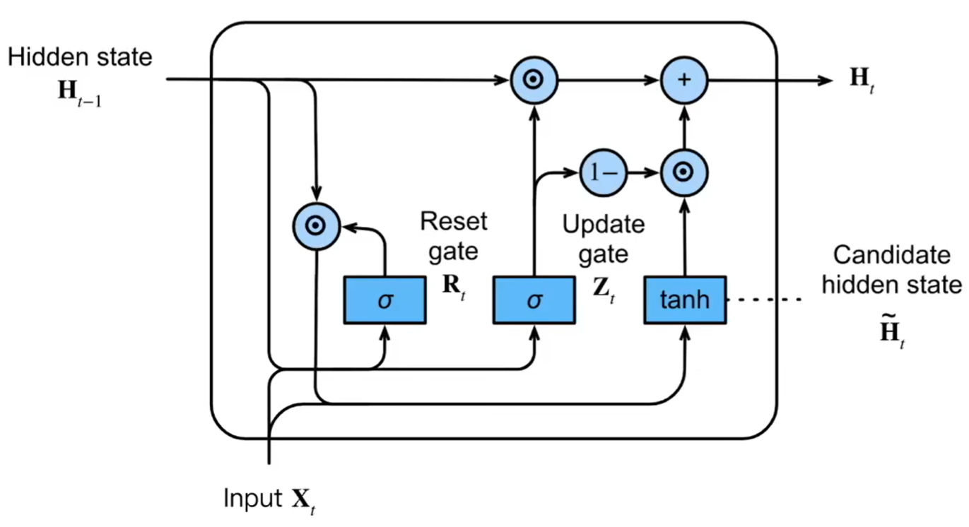
图 11.2: GRU

\[ \begin{aligned} R_t &= \sigma(X_t W_{xr} + H_{t-1} W_{hr} + b_r) \\ Z_t &= \sigma(X_t W_{xz} + H_{t-1} W_{hz} + b_z) \\ \tilde{H}_t &= \tanh(X_t W_{xh} + (R_t \odot H_{t-1}) W_{hh} + b_h) \\ H_t &= Z_t \odot H_{t-1} + (1 - Z_t) \odot \tilde{H}_t \end{aligned} \]

重置门\(R_t\)用于控制过去的隐藏状态有多少内容被用于生成当前候选隐藏状态，更新门\(Z_t\)用于控制生成当前隐藏状态时过去隐藏状态和候选隐藏状态的权重。

11.4.2 示例

import torch
import torch.nn as nn
import torch.optim as optim
import numpy as np
import matplotlib.pyplot as plt


# ------------------------------
# 1. 生成模拟数据
# ------------------------------
# 我们造一个简单的任务：输入一个时间序列（正弦+噪声），预测最后一个时刻的值
np.random.seed(42)
torch.manual_seed(42)

def generate_data(num_samples=200, seq_len=20):
    X = []
    y = []
    for _ in range(num_samples):
        freq = np.random.uniform(0.5, 1.5)
        phase = np.random.uniform(0, np.pi)
        noise = np.random.normal(0, 0.1, seq_len)
        seq = np.sin(np.linspace(0, 2 * np.pi * freq, seq_len) + phase) + noise
        X.append(seq)
        y.append(seq[-1])  # 预测最后一个点
    X = np.expand_dims(np.array(X), axis=2)  # (N, T, 1)
    y = np.expand_dims(np.array(y), axis=1)  # (N, 1)
    return torch.tensor(X, dtype=torch.float32), torch.tensor(y, dtype=torch.float32)

X, y = generate_data(num_samples=300, seq_len=30)
train_X, test_X = X[:240], X[240:]
train_y, test_y = y[:240], y[240:]


# ------------------------------
# 2. 定义 GRU 模型
# ------------------------------
class GRUNet(nn.Module):
    def __init__(self, input_size, hidden_size, num_layers, output_size,
                 dropout=0.2, bidirectional=False):
        super(GRUNet, self).__init__()
        self.hidden_size = hidden_size
        self.num_layers = num_layers
        self.bidirectional = bidirectional

        self.gru = nn.GRU(
            input_size=input_size,
            hidden_size=hidden_size,
            num_layers=num_layers,
            dropout=dropout if num_layers > 1 else 0.0,
            bidirectional=bidirectional,
            batch_first=True
        )
        # 如果是双向GRU，需要乘2
        direction_factor = 2 if bidirectional else 1
        self.fc = nn.Linear(hidden_size * direction_factor, output_size)

    def forward(self, x):
        out, h = self.gru(x)              # out: (batch, seq, hidden*direction)
        out = self.fc(out[:, -1, :])      # 取最后一个时间步的输出
        return out


# ------------------------------
# 3. 初始化模型与优化器
# ------------------------------
model = GRUNet(
    input_size=1,       # 每个时间步输入1个特征
    hidden_size=32,     # 隐层维度
    num_layers=1,       # 堆叠1层GRU
    output_size=1,      # 输出一个数（预测值）
    dropout=0.2,
    bidirectional=False  # 是否使用双向GRU
)

criterion = nn.MSELoss()
optimizer = optim.Adam(model.parameters(), lr=0.005)


# ------------------------------
# 4. 训练模型
# ------------------------------
epochs = 100
train_losses = []

for epoch in range(epochs):
    model.train()
    optimizer.zero_grad()
    output = model(train_X)
    loss = criterion(output, train_y)
    loss.backward()
    optimizer.step()

    train_losses.append(loss.item())
    if (epoch + 1) % 20 == 0:
        print(f"Epoch [{epoch+1}/{epochs}], Loss: {loss.item():.6f}")

# 绘制训练损失曲线
plt.figure(figsize=(6,4))
plt.plot(train_losses)
plt.title("Training Loss Curve")
plt.xlabel("Epoch")
plt.ylabel("MSE Loss")
plt.show()


# ------------------------------
# 5. 测试与可视化
# ------------------------------
model.eval()
with torch.no_grad():
    pred = model(test_X).squeeze().numpy()
    truth = test_y.squeeze().numpy()

plt.figure(figsize=(8,5))
plt.plot(truth, label="True")
plt.plot(pred, label="Predicted")
plt.legend()
plt.title("GRU Prediction on Test Set")
plt.show()

# 计算误差指标
mse = np.mean((pred - truth)**2)
mae = np.mean(np.abs(pred - truth))
print(f"Test MSE: {mse:.6f}, MAE: {mae:.6f}")

11.4.3 拓展

同LSTM。